Introduction into Word2Vec
The tool Word2Vec was developed by Mikolov et al. (2013). The model forms the basis for the study of Le & Mikolov (2014).
The Word2vec model is elaborated in Xin Rong (2014).
Word2Vec attempts to associate words with points in space.
The spatial distance between words describes the relation (similarity) between these words.
If one word is close to another word spatially, they are similar.
Words are represented by continuous vectors over dimensions.

Fig.1 a word vector example.
Fig.1 shows a word vector example where each word is represented by a vector of two dimensions. This figure is obtained with the following codes.
%matplotlib inline
import seaborn as sb
import numpy as np

words = ['queen', 'book', 'king', 'magazine', 'car', 'bike']
vectors = np.array([[0.1,   0.3],  # queen
                    [-0.5, -0.1],  # book
                    [0.2,   0.2],  # king
                    [-0.3, -0.2],  # magazine
                    [-0.5,  0.4],  # car
                    [-0.45, 0.3]]) # bike

sb.plt.plot(vectors[:,0], vectors[:,1], 'o')
sb.plt.xlim(-0.6, 0.3)
sb.plt.ylim(-0.3, 0.5)
for word, x, y in zip(words, vectors[:,0], vectors[:,1]):
    sb.plt.annotate(word, (x, y), size=12)
The displacement vector refers to the vector between two vectors, and it describes the relation between two words.
The displacement vectors can be used to find pairs of words following analogy relation:.
queen : king :: woman : man which should be read as queen relates to king in the same way as woman relates to man.
In algebraic formulation: $$\bar{v}{\rm queen}−\bar{v}{\rm king}=\bar{v}{\rm woman}−\bar{v}{\rm man}$$.
This analogy relation technique can be applied to e.g. question answering.
Word2Vec learns continuous word embeddings from plain text.
The word2vec model assumes the Distributional Hypothesis.
Distributional Hypothesis means that words are characterized by words they hang out with.
The word2vec model accompanied with distributional hypothesis can be applied to estimate the probability of two words occurring near each other.

Fig.2 Probability of the words appears after `Cinderella'.
For example, fig.2 shows the probability of the words appear after `Cinderella', i.e., $${\rm P}({\rm w}|{\rm Cinderella})$$.
The pumpkin, shoe, tree, prince and luck have probability of 0.1, 0.4, 0.01, 0.2 and 0.05, respectively.
The figure can be obtained with codes as following.
import pandas as pd
s = pd.Series([0.1, 0.4, 0.01, 0.2, 0.05],
              index=["pumpkin", "shoe", "tree", "prince", "luck"])
s.plot(kind='bar')
sb.plt.ylabel("$P(w|Cinderella)$")
Softmax Regression
The word2Vector model considers each word wo in turn along with a given context C
For exmaple, A vocabulary bank contains many wO and the total size is V .
one of the wO=Cinderella and C=shoe
If the context C is be given, how to predict the right wO in the vocabulary bank.
To compute a probability distribution y^ over the labels, the model use softmax regression.
The model attempts to minimize via Stochastic Gradient Descent the difference between the output distribution and the target distribution (which is a one-hot distribution which places all probability mass on the correct word).
The difference between the two distribution is measured by the cross-entropy.
The figure3 shows the neural network contains two matrics: W and W′ of dimensions V×N and N×V respectively, where V is the vocabulary size and N is the number of dimensions.
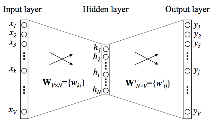
Fig.3 A simple neural network with a single hidden layer
The figure can use the following example to illustrate.
A corpus containing the following documents:
sentences = ['the king loves the queen', 'the queen loves the king',
             'the dwarf hates the king', 'the queen hates the dwarf',
             'the dwarf poisons the king', 'the dwarf poisons the queen'
Transform these documents into bag-of-indices to enable easier computation:
from collections import defaultdict

def Vocabulary():
    dictionary = defaultdict()
    dictionary.default_factory = lambda: len(dictionary)
    return dictionary

def docs2bow(docs, dictionary):
    """Transforms a list of strings into a list of lists where
    each unique item is converted into a unique integer."""
    for doc in docs:
        yield [dictionary[word] for word in doc.split()]
vocabulary = Vocabulary()
sentences_bow = list(docs2bow(sentences, vocabulary))
sentences_bow
Construct the two matrices W and W′:
import numpy as np

V, N = len(vocabulary), 3
WI = (np.random.random((V, N)) - 0.5) / N
WO = (np.random.random((N, V)) - 0.5) / V
Each row i in W corresponds to word i and each column j corresponds to the jth dimension.
print WI
Notice that W′ isn't simply the transpose of W but a different matrix:
print WO
Compute the probability of an output word given some input word.:
For example, given an input word wI, e.g. dwarf and its corresponding vector WI, what is the probability that the output word wO is hates? Using the dot product WI⋅W′TO and compute the distance between the input word dwarf and the output word hates:
print np.dot(WI[vocabulary['dwarf']], WO.T[vocabulary['hates']])
0.000336538415207
Now using softmax regression, we can compute the posterior probability P(wO|wI):
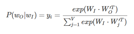
p_hates_dwarf = (np.exp(np.dot(WI[vocabulary['dwarf']], WO.T[vocabulary['hates']])) /
                       sum(np.exp(np.dot(WI[vocabulary['dwarf']], WO.T[vocabulary[w]]))
                           for w in vocabulary))
print p_hates_dwarf
0.14291402521
Updating the hidden-to-output layer weights
Word2Vec attempts to associate words with points in space.
These points in space are represented by the continuous embeddings of the words.
All vectors are initialized as random points in space, so we need to learn better positions. ??
The model does so by maximizing the equation above. The corresponding loss function which we try to minimize is E=−logP(wO|wI).
First, update the hidden-to-output layer weights.
Say the target output word is Cinderella. Given the aformentioned one-hot target distribution t, the error can be computed as tj−yj=ej, where tj is 1 iff wj is the actual output word.
So, the actual output word is Cinderella and we compute the posterior probability of P(pumpkin | tree), the error will be 0 - P(pumpkin | tree), because pumpkin isn't the actual output word.
To obtain the gradient on the hidden-to-output weights, we compute ej⋅hi, where hi is a copy of the vector corresponding to the input word (only holds with a context of a single word).
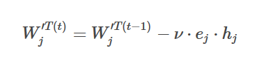
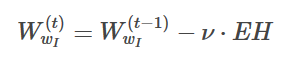
Finally, using stochastic gradient descent, with a learning rate ν we obtain the weight update equation for the hidden to output layer weights:
Assume the target word is king and the context or input word C is queen.
Given this input word we compute for each word in the vocabulary the posterior probability P(word | queen).
If the word is the target word, the error will be 1 - P(word | queen); otherwise 0 - P(word | queen).
Finally, using stocastic gradient descent we update the hidden-to-output layer weights:
target_word = 'king'
input_word = 'queen'
learning_rate = 1.0

for word in vocabulary:
    p_word_queen = (np.exp(np.dot(WO.T[vocabulary[word]], WI[vocabulary[input_word]])) /
                    sum(np.exp(np.dot(WO.T[vocabulary[w]], WI[vocabulary[input_word]]))
                        for w in vocabulary))
    t = 1 if word == target_word else 0
    error = t - p_word_queen
    WO.T[vocabulary[word]] = (WO.T[vocabulary[word]] - learning_rate *
                              error * WI[vocabulary[input_word]])
print WO
Updating the input-to-hidden layer weights
In order to update the input-to-hidden layer weight, backprppagating the prediction error to the input-to-hidden weights.
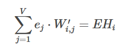
Firstly, compute EH(N dimensional vector). EH is the sum of the hidden-to-output vectors for each word in the vocabulary weighted by their prediction error:
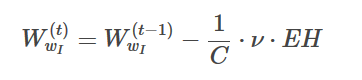
Secondly, using the learning rate ν we update the weights using:
The formula can be obtained with codes as following.
WI[vocabulary[input_word]] = WI[vocabulary[input_word]] - learning_rate * WO.sum(1)
The probability of king given queen will grow up If recomputing the probability of each word given the input word queen
for word in vocabulary:
    p = (np.exp(np.dot(WO.T[vocabulary[word]], WI[vocabulary[input_word]])) /
         sum(np.exp(np.dot(WO.T[vocabulary[w]], WI[vocabulary[input_word]]))
             for w in vocabulary))
    print word, p
king 0.135793930736
dwarf 0.143640274055
queen 0.141911808054
poisons 0.144219025126
loves 0.14461048255
the 0.1457335424
hates 0.144090937079
Multi-word context
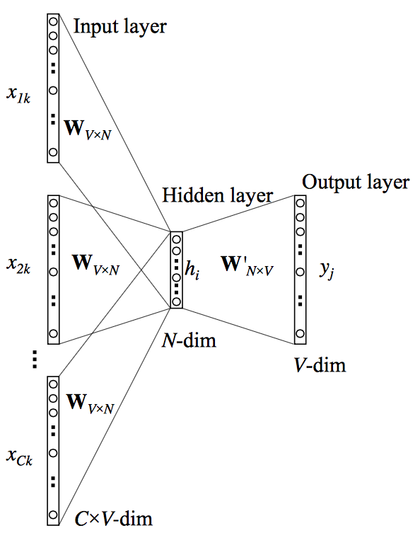
Fig.4 CBOW architecture of Word2Vec.
To simply copy the input vector to the hidden layer, the article assumes that the context C was only a single input word.
If the context C comprises multiple words, taking the mean of their input vectors as our hidden layer, instead of copying the input vector.
The update functions remain the same except that for the update of the input vectors. Therefore, updating to each word in the context C:
Assuming the target word is king. The context consists of two words: queen and loves.
The formula can be obtained with codes as following.
target_word = 'king'
context = ['queen', 'loves']
Firstly, taking the average of the two context vectors:
h = (WI[vocabulary['queen']] + WI[vocabulary['loves']]) / 2
Secondly, applying the hidden-to-output layer update:
for word in vocabulary:
    p_word_context = (np.exp(np.dot(WO.T[vocabulary[word]], h)) /
                            sum(np.exp(np.dot(WO.T[vocabulary[w]], h)) for w in vocabulary))
    t = 1 if word == target_word else 0
    error = t - p_word_context
    WO.T[vocabulary[word]] = WO.T[vocabulary[word]] - learning_rate * error * h
print WO
Finally, updating the vector of each input word in the context:
for input_word in context:
    WI[vocabulary[input_word]] = (WI[vocabulary[input_word]] - (1. / len(context)) *
                                  learning_rate * WO.sum(1))
h = (WI[vocabulary['queen']] + WI[vocabulary['loves']]) / 2
for word in vocabulary:
    p = (np.exp(np.dot(WO.T[vocabulary[word]], h)) /
               sum(np.exp(np.dot(WO.T[vocabulary[w]], h)) for w in vocabulary))
    print word, p
king 0.129518690596
dwarf 0.145150475243
queen 0.143019721408
poisons 0.145122173218
loves 0.146255939585
the 0.146300899102
hates 0.144632100847
Paragraph Vector
The Paragraph Vector was described in Le & Mikolov (2014).
The Paragraph Vector model attempts to learn fixed-length continuous representations from variable-length pieces of text.
These representations combine bag-of-words features with word semantics and can be used in all kinds of NLP applications.
Similar to the Word2Vec model, the Paragraph Vector model also attempts to predict the next word in a sentence.
The only real difference, as the paper itself states, is with the computation of h.
Where in the original model h is based solely on W, in the new model (figure 5) another matrix called D is added and D represents the vectors of paragraphs:
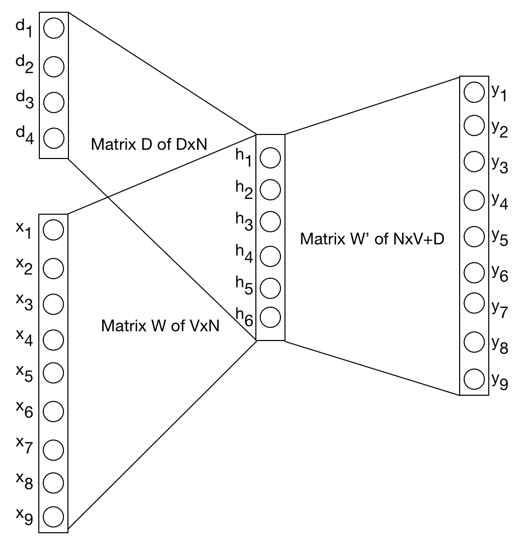 Fig.5 the Paragraph Vector model
According to this paper, a paragraph token can be thought of another word token except that all paragraph vectors are unique, whereas word tokens share their vector representations among different contexts.
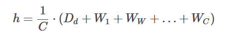
To compute h by concatenating or averaging a paragraph vector d with a context of word vectors C:
The weight update functions are the same as in Word2Vec except that the updating of the paragraph vectors.
This first model is called the Distributed Memory Model of Paragraph Vectors. Le & Mikolov present another model called Distributed Bag of Words Model of Paragraph Vector.
This model ignores the context C and attempts to predict a randomly sampled word from a randomly sampled context window.
Having a more detailed look at the DM Model.
In addition to the matrix W, matric D with dimensions P×N need to randomly initialized .
P is the number of paragraphs or whatever textual unit we use, and N is the number of dimensions.
V, N, P = len(vocabulary), 3, 5
WI = (np.random.random((V, N)) - 0.5) / N
WO = (np.random.random((N, V)) - 0.5) / V
D =  (np.random.random((P, N)) - 0.5) / N
Say out corpus consists of the following five sentences (paragraphs):
sentences = ['snowboarding is dangerous', 'skydiving is dangerous',
             'escargots are tasty to some people', 'everyone loves tasty food',
             'the minister has some dangerous ideas']
Firstly, convert the sentences into a vectorial BOW representation:
vocabulary = Vocabulary()
sentences_bow = list(docs2bow(sentences, vocabulary))
sentences_bow
[[0, 1, 2],
[3, 1, 2],
[4, 5, 6, 7, 8, 9],
[10, 11, 6, 12],
[13, 14, 15, 8, 2, 16]]
After that, compute the posterior probability for each word in the vocabulary given the concatenation and averaging of the first paragraph and the context word snowboarding.
target_word = 'dangerous'
h = (D[0] + WI[vocabulary['snowboarding']]) / 2
learning_rate = 1.0

for word in vocabulary:
    p = (np.exp(np.dot(WO.T[vocabulary[word]], h)) /
                      sum(np.exp(np.dot(WO.T[vocabulary[w]], h)) for w in vocabulary))
    t = 1 if word == target_word else 0
    error = t - p
    WO.T[vocabulary[word]] = (WO.T[vocabulary[word]] - learning_rate * error * h)
print WO
[[-0.01599941 0.02135301 0.0927715 -0.00565041 -0.00361651 -0.01454073
0.02333261 0.00211833 0.00254255 0.02315315 -0.01917578 0.00724787
-0.00117272 -0.02043504 0.00593186 -0.0166333 -0.0306218 ]
[ 0.0089237 -0.00397806 -0.13199195 0.02555059 -0.02095756 -0.00978333
0.01561624 0.03603476 -0.02114407 -0.01552016 0.01289922 0.00119743
-0.00112818 0.01708133 0.00765248 0.02442374 0.01109005]
[-0.01205008 -0.03123478 0.05878695 0.02615259 -0.01025209 -0.00442044
0.00311309 0.01554668 0.02344194 0.00602561 -0.03117694 0.01368817
0.00858936 -0.00223242 -0.01141366 -0.01719967 -0.01400046]]
Finally, computing the error and update the hidden-to-output layer weights.
EH = WO.sum(1)
WI[vocabulary['snowboarding']] = WI[vocabulary['snowboarding']] - 0.5 * learning_rate * EH
D[0] = D[0] - 0.5 * learning_rate * EH
Experiments
Le & Mikolov evaluate and investigate the performance of the paragraph vectors on a number of different tasks. I will briefly discuss them here.
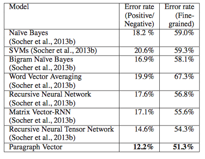
Sentiment Analysis
In the first experiment, the authors address the task of sentiment analysis. They make use of the Stanford Sentiment Treebank Dataset which is a manually annotated data set containing 11855 sentences taken from the movie review site Rotten Tomatoes. Each sentence in the data set has been assigned a label on a scale of negative to positive. The task is to predict these labels.
Le & Mikolov train Paragraph Vectors using both the DM Model and the DBOW model. These two representations are concatenated for each training instance and fed to a Logistic Regression classifier that makes a prediction for each unseen test sentence. In table compares the performance of the model to a number of different models:
Tab1 The error rate of sentiment analysis in different model
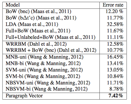
Le & Mikolov then move on beyond the sentence level and evaluate their model on the IMDB data set. Training and testings follows the same procedure as before. The table 2 suggest a strong improvement compared to the other reported models:
Tab2 The error rate of sentiment analysis in different model beyond the sentence level
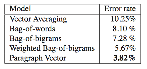
Information Retrieval
The authors then turn to an experiment in Information Retrieval. They develop a task in which the goal is to predict which of three paragraphs isn't the result of the same query. They construct a data set on the basis of the search results of a search engine. For each query they create a triplet of paragraphs: two paragraphs are results from the same query and one is randomly sampled from the rest of the collection (result from a different query). The pairwise distances between each member of a triplet, should then reflect which two results belong to the same query and which snippet is the outlier. The table 3 shows quite convincingly how well the paragraph vectors are able to perform on this task compared to the other methods:
Tab3 The error rate of information retrieval in different models
General remarks
The ease with which the model can be applied to text pieces of variable length is perhaps the strongest advantage of the model.
Availability of code / experimentation details
No implementation was available (even not to the second author, which led to some serious doubts about the reproducability of the results:
The authors report a number of hyperparameters in the paper, such as the window size and the number of dimensions of the vectors. However, some crucial parameters weren't mentioned (such as the use of hierarchical softmax verus negative sampling). Again, in order to reproduce the results, the authors must specify in much greater detail how they performed the experiments.
Reference: http://nbviewer.jupyter.org/github/fbkarsdorp/doc2vec/blob/master/doc2vec.ipynb